


SolarFarmer Model
Modelling methodology, assumptions & key parameters
SolarFarmer Calculation Methodology
SolarFarmer is DNV’s advanced PV design & simulation API for solar design and yield assessment. It combines detailed spatial modelling with a physics-based calculation engine to simulate PV system performance across a wide range of climates, topographies, and system configurations — including bifacial modules and complex AC collection systems.
The model operates with a modular architecture that models the physics of how energy is generated, and connected to the grid from Solar Panel to Inverter. Each step in the energy chain is represented by a specific calculation stage, grounded in validated engineering methods.
The SolarFarmer model is fully documented in the SolarFarmer Technical Documentation. The sections below provide an overview of each stage with direct links to the relevant documentation.
Irradiance Modelling
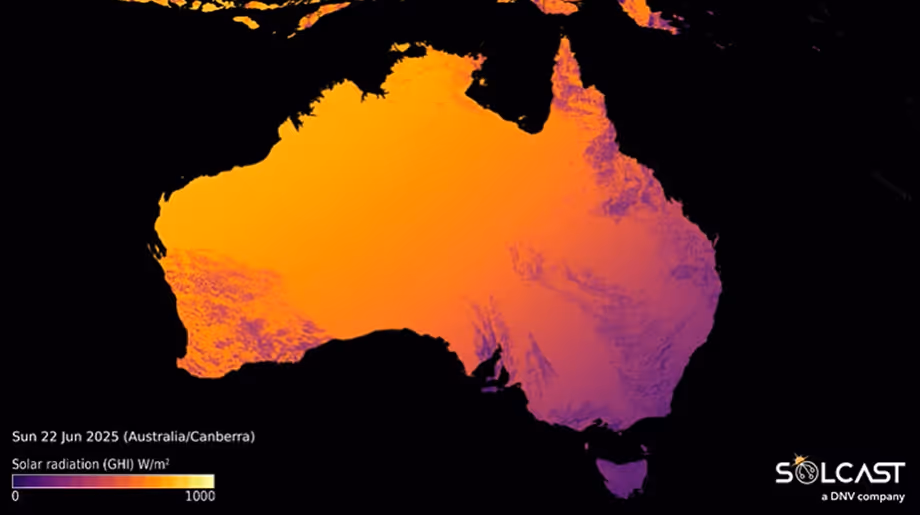
SolarFarmer takes irradiance inputs from either ground-based measurements (such as on-site pyranometers) or satellite-derived datasets from any provider, not limited to Solcast. It then calculates how this irradiance is distributed at the PV system level. This includes transposition to the plane of array, adjustments for tilt and shading, and modifiers such as soiling, incidence angle, spectral effects, and bifacial gain. The result is a detailed estimate of insolation - the solar energy received per unit area on the PV modules over a given time period.
- Input Data
Supports ground-based and satellite inputs (GHI, DNI, diffuse), plus meteorological data such as temperature and wind. - Tilt & Orientation
Applies established transposition models (e.g. Perez) to calculate irradiance on tilted array surfaces. - Far & Near Shading
Shading is calculated using the Light & Shade hemicube model, which resolves both beam and diffuse components with sky-dome subdivision. - Soiling, IAM & Spectral Effects
Models additional modifiers including soiling accumulation on modules, incidence angle modifier (IAM) behaviour, and spectral mismatch between incident irradiance and module spectral response. - Bifacial Irradiance
Models rear-side irradiance using view factors, albedo, and module elevation, with support for spatially varying ground reflectance. - Inputs for Module Performance
Converts irradiance outputs into effective irradiance and cell temperature inputs for DC-side modelling.
The complete irradiance modelling workflow is documented in the calculation reference.
Conversion (DC-side)
This stage simulates how modules convert plane-of-array irradiance into DC electricity, considering IV-curve behaviour, temperature effects, mismatch, and light-induced degradation (LID)
- Array Nominal Energy
Defines the baseline module output at standard test or nominal operating conditions. - Module Performance Models
Implements either a single-diode physical model or empirical IV curve models, depending on available manufacturer data.” - Temperature & Irradiance Effects
Applies module temperature coefficients and irradiance adjustments to refine output under real operating conditions. - Mismatch & Optimisers
Represents mismatch losses arising from shading, orientation differences, or module binning, with optional modelling of power optimizer behaviour at module or string level. - Light-Induced Degradation (LID)
Applies module-specific LID factors to reflect early degradation effects after installation. - DC Collectors
Simulates electrical resistance and voltage drop across the DC collection system.
All DC-side conversion effects are described in detail in the technical documentation.
Inverter Modelling
The theoretical basis section documents the underlying mathematical models and references that support SolarFarmer’s methodology.
- Efficiency & Curves
Incorporates manufacturer-supplied inverter efficiency maps across voltage and load ranges. - Operating Windows
Models inverter startup, MPPT voltage/current ranges, clipping behaviour, and over-power conditions. - Tare & Standby Losses
Includes non-generation consumption such as night-time tare losses.
Inverter modelling assumptions and formulas are set out in the SolarFarmer Calculation Reference.
AC Collection System
The AC collection model represents the electrical network from inverters to grid connection, capturing resistive losses, transformer behaviour, and availability factors.
- AC Collectors
Configures cables, transformers, and auxiliary systems at multiple voltage levels. - Availability & Grid Limit
Applies I²R, transformer, curtailment, and availability losses across the AC network. - Grid Connection Limit
Enforces power export caps or interconnection constraints at the point of grid connection.
See the AC collection section of the technical documentation for detailed parameters.
Summary Results
SolarFarmer produces aggregated results and performance indicators across multiple system levels and timeframes.
- Aggregation
Generates results by component (string, inverter, site) and across intervals (hourly, daily, monthly, annual). - Performance Ratio (PR)
Calculates monthly and annual PR, normalised to reference irradiance and adjusted for system losses.
Output Files
SolarFarmer generates timestamped time-series outputs in standard formats (CSV, JSON) for integration into analysis workflows, locally or via the cloud.
- Time-Series Outputs
CSV-based outputs including timestamped irradiance, module temperature, DC/AC power, and loss categories. - Cloud Outputs
Compressed results packages with CSV and JSON formats for easy portfolio integration.
SolarFarmer vs. PVsyst
SolarFarmer and PVSyst are both widely used in PV yield assessment, but they differ in several aspects of methodology and model scope. In particular, SolarFarmer applies its own approaches to terrain representation, shading calculations (via the Light & Shade hemicube model), bifacial energy capture, and treatment of loss mechanisms.
For a detailed side-by-side description of these differences, see the full documentation here in the SolarFarmer vs. PVSyst differences guide.
Theory & References
The theoretical basis section documents the underlying mathematical models and references that support SolarFarmer’s methodology.
- Theoretical Basis
Explains the mathematical models underlying irradiance, thermal, and electrical calculations. - Reference Documents
Bibliography of peer-reviewed papers, standards, and models that underpin SolarFarmer’s methodology.
Try the Solcast API
Solcast takes on the many challenges of producing live and forecast solar data, so that you don’t have to. That means making the data easy to access, validate and integrate. We provide instant access to live and forecast data products via this web interface, which is free to try. These include direct estimates of global, direct and diffuse solar radiation, as well as PV power output.