Operating a solar forecast under a penalty regime: what we've learned across multiple markets

The operating conditions of your market, particularly its regulatory penalty regime, define the risk threshold and consequences of forecasting error. Many markets are increasing the rigour of their forecasting standards through tighter error bands or higher penalties. As renewables account for a growing share of generation in a market, the variability that system operators must manage also increases. Operators not yet working under imbalance charges, capacity obligations or market-operator submission rules can reasonably expect to face them before long. Forecast accuracy therefore has an increasingly direct effect on plant revenue.

Our work with customers spans dozens of forecasting regimes, from five-minute submissions to day-ahead forecasts. We support asset operators, grid operators and regulatory authorities, giving us direct experience of how new regimes are designed, introduced and refined. In some markets, we have also helped shape the forecasting arrangements themselves, including DNV’s role as the default solar and wind forecaster for New Zealand’s Electricity Authority

Across these markets, the same practical questions recur:

what site adaptation can improve, how operators can use P90, P75, P25 and P10 forecasts to manage risk, and how curtailment and availability data should be handled.

The answers vary with the market rules, PPA obligations and imbalance arrangements, but the commercial principle is the same: the difference between forecast and delivery can affect revenue and, ultimately, an operator’s profit and loss.

Why train your site model on operational data

For solar, training on a plant's own generation data is how a model learns the practical behaviour and operational realities that a theoretical power model forecast can’t capture. Inverter clipping caps the top of a sunny afternoon at a level set by the plant's DC:AC ratio, which a naïve forecast has no knowledge of. Complex or localised shading reduces production at a level of detail a typical pvlib model would not resolve.  By combining the plant's SCADA and site measurements with multiple weather data sources and satellite-derived irradiance, the model learns the nuances of how local meteorological and physical effects translate into generation. Those nuances cannot be practically represented in a purely theoretical model. The result is a megawatt forecast tuned to the asset.

Site adaptation cannot correct an inaccurate weather forecast. If the weather model is wrong about tomorrow’s conditions, training on historical generation will not make that weather forecast more accurate. It improves the conversion from forecast irradiance to power by accounting for how the plant actually behaves. This reduces one source of error, but it does not remove the uncertainty in the underlying weather forecast.

Using probability ranges to size a bid

The value of uncertainty information lies in the decisions it enables. A central forecast provides an expected outcome, but not the likelihood of other plausible outcomes. Two forecasts can have the same expected generation while carrying very different levels of upside and downside risk. Probability bands make those differences visible, helping operators make decisions that reflect both the expected outcome and the risks around it.

‍

A bid based only on the central estimate would be the same in both cases, despite the greater risk represented by the wider range. Probability-of-exceedance values allow the operator to account for that difference when deciding what to nominate.

A probabilistic forecast describes uncertainty using values with different probabilities of exceedance. P90 is a relatively conservative estimate with a 90% probability of being exceeded, while P10 is a higher estimate with only a 10% probability of being exceeded. The range between them shows the spread of plausible generation outcomes. P75 and P25 provide additional points within that range, allowing operators to make more nuanced decisions where the most conservative or most ambitious estimates do not match their risk appetite. Together, these values allow operators to choose a nomination that reflects both their risk appetite and the relative cost of over- and under-delivery.  

When using these values to size a bid, the following four steps can help:

1. Read the range, not only the central estimate. The central estimate is the best single estimate; the spread between P10 and P90 indicates the model’s uncertainty for that interval. A narrow band and a wide band are different operating situations even when the central estimate is identical.
2. ‍Establish your risk asymmetry. Determine what an over-delivery costs relative to an under-delivery. In most markets, these are not symmetric. Also understand how the regime treats over- and under-delivery, and whether decisions made further ahead limit the positions available closer to delivery. Understanding these factors allows operators to match their power forecast to an acceptable risk range in their forecast bids. ‍
3. Select the probability-of-exceedance value that matches your risk appetite. In forecasting regimes that penalise shortfall more heavily, a more conservative forecast can protect against the expensive downside. P75 and P25 provide intermediate options where P90 or P10 are too conservative or too aggressive for the exposure being managed. ‍
4. Size the bid accordingly, and re-size as the range narrows. Typically, the P90–P10 range narrows between the day-ahead forecast and the final bid-submission deadline as more recent data become available.

These probability ranges depend on the quality of the underlying weather forecasts, uncertainty modelling and power model. For a site-trained power model, that quality also depends on correctly identifying periods when output was restricted by curtailment or reduced availability.

Curtailment and availabiilty. Connecting plant conditions to the power forecast.

A power measurement shows what the plant produced, but not necessarily what it was capable of producing. Lower output may reflect the weather, curtailment, reduced availability or genuine underperformance. Without additional plant data, a forecasting model cannot reliably distinguish between them.

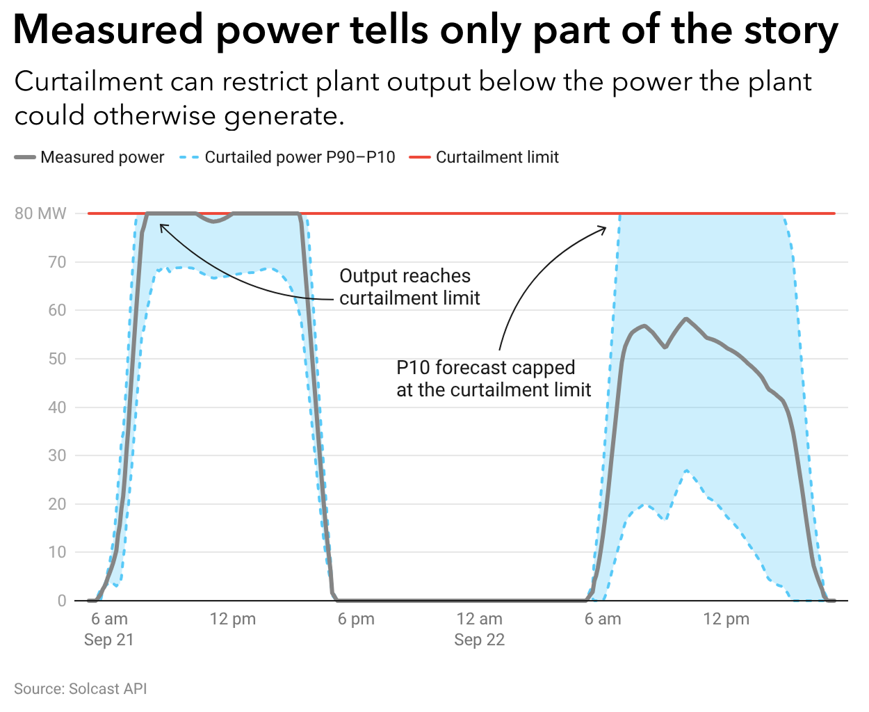
Curtailment and reduced-availability periods therefore need to be labelled or excluded from training data. Otherwise, the model may treat restricted production as normal plant behaviour and forecast too little power when similar conditions occur again.

The same information matters in real time. Short-term forecasts incorporating the most recent measurements can be distorted if those measurements reflect curtailment or reduced availability rather than the plant’s production potential. Providing expected curtailment and availability schedules allows the forecast to distinguish between the power the plant could generate and the restrictions currently limiting its output.

Persistent characteristics, such as long-term shading, belong in the site model. Temporary events, such as an outage or missed cleaning cycle, should not be treated as normal plant performance.

How penalty regimes differ

The forecasting techniques described so far are broadly the same no matter where your plant operates. What changes between markets is what the forecast is measured against, and what an error costs. Across the markets we work in, regimes fall into six broad groups.

1. Imbalance managed centrally. Under legacy feed-in tariffs and must-purchase schemes, the generator sells everything at a fixed price and the offtaker or consumer absorbs the imbalance. Forecasting is left to the system operator. Regimes like these are gradually disappearing as support schemes expire and renewable penetration increases. Markets are increasingly shifting forecasting and balancing responsibility from system operators to generators and their trading counterparties.
2. Market-priced imbalance settlement. In many European markets, the generator, or its aggregator, sits in a balance group, nominates a schedule and settles any deviation at an imbalance price derived from costs of peaking and balancing sources needed to keep the system in balance. German TSOs describe this as a price rather than a penalty, and a deviation that happens to help the system can earn money as well as cost it. Single imbalance pricing is now the EU default under the harmonized imbalance settlement rules that implement the Electricity Balancing Guideline. The cost of an error therefore depends on its size and on whether the system was in under-supply or over-supply at the time.
3. Tolerance bands with escalating charges. The regulator sets tolerance bands around the schedule and charges more as the deviation moves into each wider band. These regimes tend to appear where there is no established balancing market to price imbalance, or where a regulator prefers to set the charges directly. Grids in India, China and Turkey all use versions of this approach, and the rules can differ even within one country. In China, each regional grid sets its own penalty metric. Central China Grid, for example, bases its penalty on mean absolute error (MAE), while East China Grid uses squared percentage error (SPE). The exposure also depends on what error is measured against (available capacity, scheduled generation or installed capacity), whether plants are assessed individually or in aggregate, and also if over- and under-delivery are treated alike. Where under-forecasting is penalised more heavily than over-forecasting, nominating below the central forecast moves more of your misses onto the cheaper side.
4. Compliance with dispatch instructions. In centrally-dispatched markets, the plant's obligation is to follow the dispatch target issued by the system operator. The plant's forecast typically influences those targets through the available generation it reports to the operator. While the treatment of deviations differs between markets, exposure generally arises when actual output diverges from the dispatch instruction rather than from a forecast schedule or nominated position. ERCOT (Texas, USA), CAISO (California, USA), and AESO (Alberta, Canada) all follow this broad approach, each with its own tolerances, pricing arrangements and exemptions. In these markets, accurate curtailment and availability data are a large part of managing that exposure.
5. Cost allocation based on frequency impact. This approach allocates regulation reserve costs according to participants’ contribution to system frequency. In Australia’s National Electricity Market, Frequency Performance Payments replaced the former Causer Pays framework in 2025. The arrangement assigns positive or negative payments depending on whether a facility’s deviations help or harm system frequency, while using those contributions to allocate regulation reserve costs. ‍
6. Additional payments for forecast accuracy. Some markets add a direct accuracy incentive to their underlying market arrangements. In South Korea, renewable generators enrolled in the forecasting incentive programme receive an additional payment when their forecast error remains within a set threshold, with a higher payment for meeting a tighter threshold.

PPAs and tender documents add another layer of forecasting obligations, regardless of the market arrangements a project operates under. Availability guarantees and minimum generation commitments may carry their own charges for missed output, and contractual exposure can sometimes outweigh the regulatory exposure.

These arrangements often overlap. A solar farm in Great Britain may have its imbalance settled by its offtaker, with the cost passed back through its PPA. Responsibility for the forecast itself can also vary. In New Zealand, each wind and solar site receives a centrally-procured forecast, but generators may use their own forecast if it meets the required performance standards. Operators therefore need to understand what they must submit, how deviations are treated and where the financial exposure ultimately sits.

Forecasting to the rules of your market

Each regime sets its own submission requirements, from forecast resolution and horizon to bid submission deadlines and how often a position can be revised. Meeting them takes forecast data that is reliable and arrives in time to act on.

The Solcast API issues updated forecasts every 5 to 15 minutes, using the latest satellite-derived irradiance and weather-model data. Forecasts extend from five minutes ahead to 14 days, at intervals ranging from five to 60 minutes. They can be trained on a site’s own measurements and incorporate curtailment and availability schedules. Selected plans also provide P90, P75, P25 and P10 probability-of-exceedance values alongside the central forecast. DNV is the default solar and wind forecaster for several grid operators, including New Zealand's Electricity Authority, and works with asset operators across these regimes.

If you would like to compare your current forecast against a site-trained probabilistic forecast on your own generation data, speak with our team today.